Contents
- Optimization and search
- Evolutionary Algorithms
- Representation, Mutation, and Recombination
- Fitness, Selection and Population Management
- Popular Evolutionary Algorithm Variants
- Working with Evolutionary Algorithms
- Hybridisation with Other Techniques
- Multiobjective Evolutionary Algorithms
- Machine learning and single-layer neural networks
- Multi-Layer Network
- Reinforcement Learning
Optimization and search
Finding the best solution(max/min) to a problem on a fitness-landscape.
- Continuous Optimization is the mathematical discipline which is concerned with finding the maxima and minima of functions, possibly subject to constraints.
- Discrete Optimization is the activity of looking thoroughly in order to find an item with specified properties among a collection of items.
Optimization Methods
Discrete
Exhaustive search(Brute-force search)
- Test all possible solutions, pick the best
- Guaranteed to find the optimal solution
- Possible implementation:
def exhaustive_search_max(function, range):
  solution = [range[0], function(range[0])]
  for x in range:
      if function(x) > solution[1]:
          solution = x, function(x)
  return solution
Greedy search
- Only test one solution
- Makes locally optimal choices, taking the first and “best” solution.
- TSP example: always go to the nearest city
Hill climbing
- Pick a solution as the current best(random)
- Compare to neighbor, switch if better
- Only finds local optimum, not global optimum!
Simulated annealing
- Set an initial temperature T
- Pick an initial solution
- Repeat:
- Pick a solution neighboring the current solution
- If the new one is better, keep it
- Otherwise, keep the new one with probability p
- p depends on the difference in quality and the temperature. High temp -> high p (more randomness)
- Reduce T
Continuous
Gradient descent/ascent
- Finding the gradient of the function and move towards the preferred direction.
- \(x^{(k+1)} = x^{(k)} + \gamma \nabla f(x^{(k)})\)
- Algorithm:
- Start with a point (guess)
- Repeat
- Determine a descent direction
- Choose a step
- Update
- Until stopping criterion is satisfied
- Possible Gradient ascent implementation:
def gradient_ascent(function, derivative, gamma, x , precision):
  dx = gamma * derivative(x)
  while abs(dx) > precision:
      y = function(x)
      x += dx
      dx = gamma * derivative(x)
  return x,function(x)
Exploitation and Exploration
- Search methods should combine:
- Trying completely new solutions (like in exhaustive search) => Exploration
- Trying to improve the current best solution by local search => Exploitation Combining these are more likely to give the global optima.
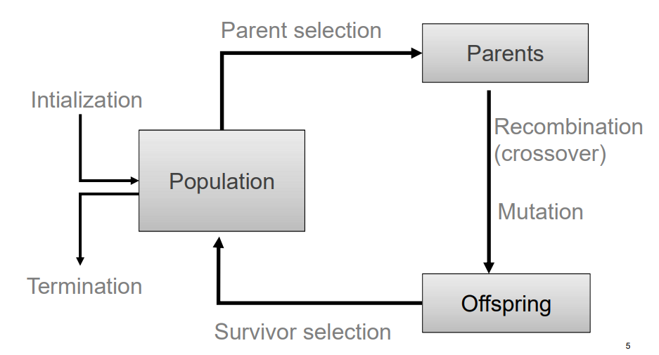
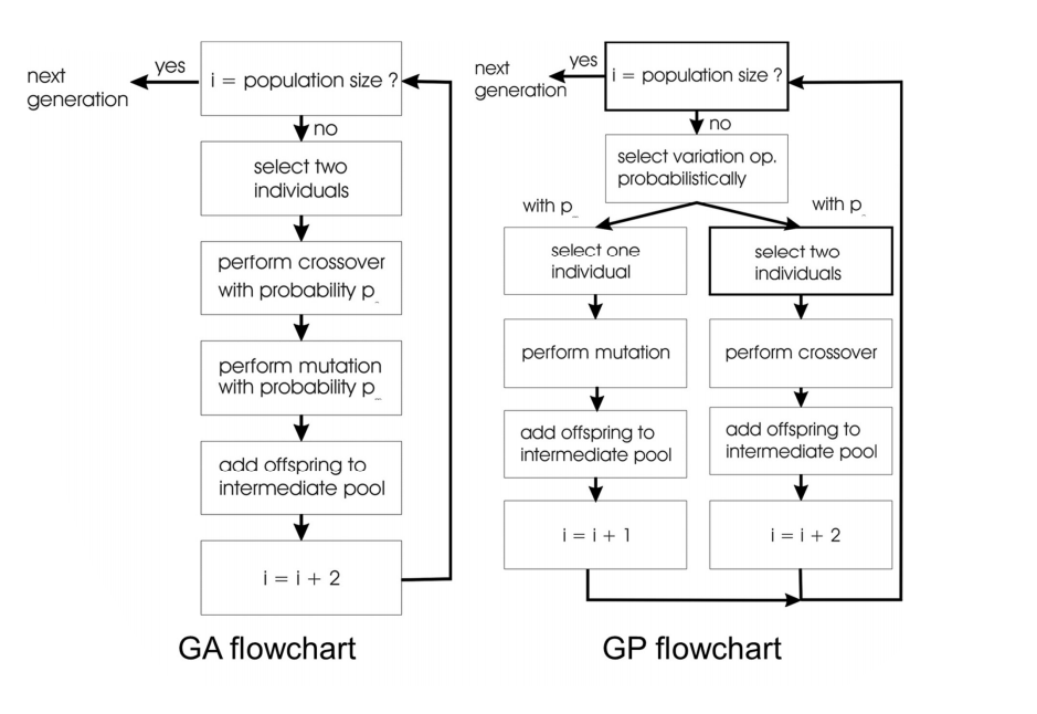
Evolutionary Algorithms
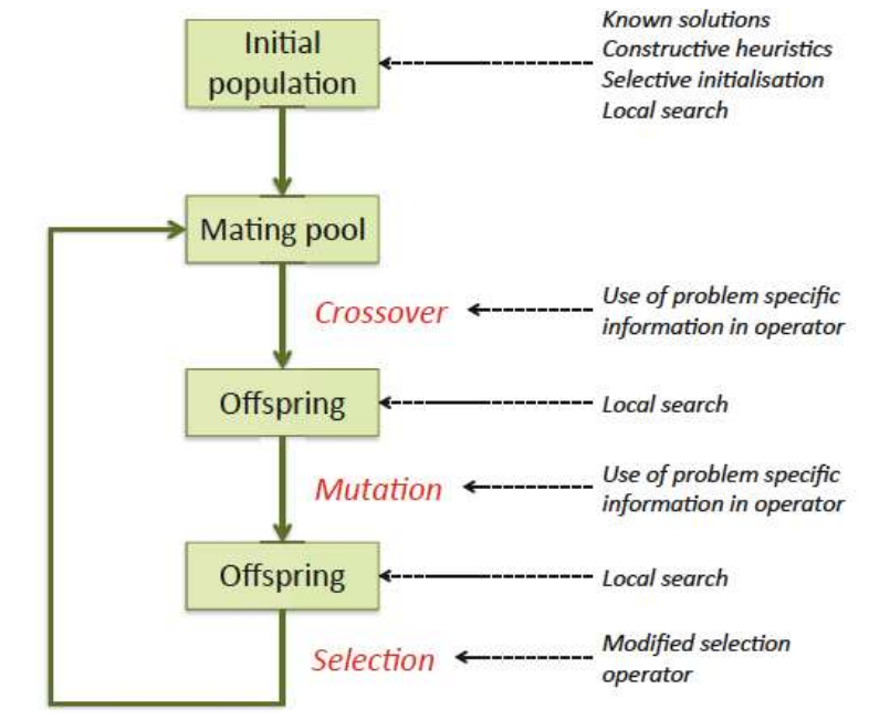
General scheme:
Psudo-code
BEGIN
	INITIALIZE population with random candidate solutions;
	EVALUATE each candidate;
	REPEAT UNTIL(TERMINATION CONDITION is satisfied) DO
		1 SELECT parents;
		2 RECOMBINE pairs of parents;
		3 MUTATE the resulting offspring;
		4 EVALUATE new candidates;
		5 SELECT individuals for the next generation;
	OD
END
The two pillars of evolution
Pushing towards novelty
Increasing population diversity by genetic operators
- mutation
- recombination
Pushing towards quality
Decreasing population diversity by selection
- of parents
- of survivors
Terminology
Evaluation(fitness) function
- Represents the task to solve
- Provides basis for comparison of fitness for each phenotype
- Assigns a single real-valued fitness to each phenotype
Population
- The candidate solutions of the problem
- The population is evolving, not the individuals
- Selection operators act on population level
- Variation operators act on individual level
Selection mechanism
- Identifies individuals
- to become parents
- to survive
- Pushes population towards higher fitness
- Parent selection is usually probabilistic
- high quality solutions more likely to be selected than low quality, but not guaranteed due to local optima issues(stochastic nature)
Survivor selection
- N old solutions + K new solutions (offspring) -> N individuals (new population)
- Often deterministic:
- Fitness based: e.g., rank old population + offspring and take best
- Age based: make N offspring and delete all old solutions
- Sometimes a combination of stochastic and deterministic (elitism)
Variation operators
- Role: to generate new candidate solutions
- Usually divided into two types according to their arity (number of inputs to the variation operator):
- Arity 1 : mutation operators
- Arity >1 : recombination operators
- Arity = 2 typically called crossover
- Arity > 2 is formally possible, seldom used in EA
Mutation
- Role: cause small, random variance to a genotype
- Element of randomness is essential and differentiates it from other unary heuristic operators
- Importance ascribed depends on representation and historical dialect:
- Binary Genetic Algorithms – background operator responsible for preserving and introducing diversity
- Evolutionary Programming for continuous variables – the only search operator
- Genetic Programming – hardly used
Recombination
- Role: merges information from parents into offspring
- Choice of what information to merge is stochastic
- Hope is that some offspring are better by combining elements of genotypes that lead to good traits
Initialisation
- Initialisation usually done at random
- Need to ensure even spread and mixture of possible allele values
- Can include existing solutions, or use problem-specific heuristics, to “seed” the population
Termination
- Termination condition checked every generation
- Reaching some (known/hoped for) fitness
- Reaching some maximum allowed number of generations
- Reaching some minimum level of diversity
- Reaching some specified number of generations without fitness improvement
Representation, Mutation, and Recombination
- Most common representation of genomes:
- Binary
- Integer
- Real-Valued or Floating-Point
- Permutation
- Tree
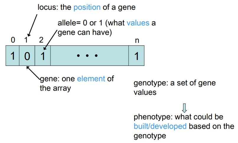
Binary Representation
- Genotype consists of a string of binary digits
- Mutation by altering each gene independently with a probability(mutation rate) \(p_m\)
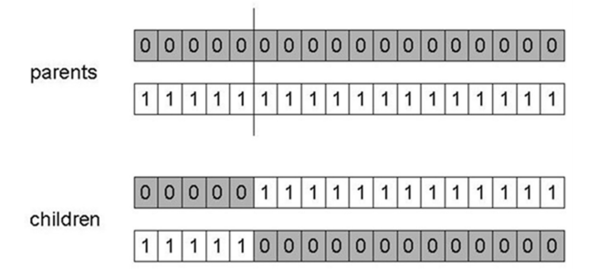
- 1-point crossover splits combines a part of each parent on a random spot:
- n-point crossover splits along n-points and recombines:
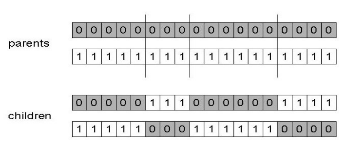
- Uniform crossover assigns a ‘head’ to one parent, ‘tail’ to the other and randomly chooses genes from each
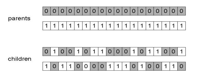
- Crossover is explorative, creates big diversion in between the parents
- Mutation is exploitative, creates random small diversion staying close to the possible optima
Integer Representation
- Could be integer variables or categorical values from a set.
- N-point / uniform crossover operators work
- Extend bit-flipping mutation to make:
- “creep” i.e. more likely to move to similar value
- Adding a small (positive or negative) value to each gene with probability \(p\)
- Random resetting (esp. categorical variables)
- With probability \(p_m\) a new value is chosen at random
- “creep” i.e. more likely to move to similar value
Real-Valued or Floating-Point
- General scheme of floating point mutations
- \(\overline{x} = \langle x_1, ..,x_l \rangle \rightarrow \overline{x}’ = \langle x_1’, .., x_l’ \rangle\)
- \(x_i, x_i’ \in [LB_i, UB_i]\)
- Uniform Mutation: \(x_i’\) drawn randomly from \([LB_i,UB_i]\)
- Analogous to bit-flipping (binary) or random resetting (integers)
- Nonuniform Mutation:
- Most common method is to add random deviate to each variable separately, taken from \(N(0,\sigma)\) Gaussian distribution and then curtail to range \(x_i’ = x_i + N(0,\sigma)\)
- Standard deviation \(\sigma\), mutation step size, controls amount of change (2/3 of drawings will lie in range \((- \sigma \rightarrow + \sigma))\)
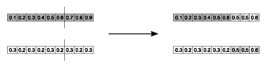
- Crossover operators:
- Discrete recombination:
- each allele value in offspring z comes from one of its parents \((x,y)\) with equal probability: \(z_i\) = \(x_i\) or \(y_i\)
- Could use n-point or uniform
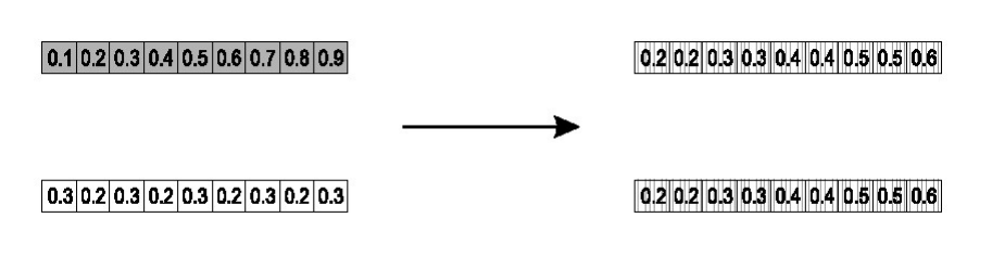
- Intermediate recombination:
- exploits idea of creating children “between” parents (hence a.k.a. arithmetic recombination)
- \(z_i = \alpha x_i + (1-\alpha)y_i\) where \(\alpha:0\leq\alpha\leq1\)
- The parameter \(\alpha\) can be:
- constant: \(\alpha = 0.5 \) -> uniform arithmetical crossover
- variable (e.g. depend on the age of the population)
- picked at random every time
- Simple arithmetic crossover
- Parents: \(\langle x_1, ..,x_n \rangle, \langle y_1, ..,y_n \rangle\)
- Pick a random gene (k) after this point mix values
- Whole arithmetic crossover
- Parents: \(\langle x_1, ..,x_n \rangle, \langle y_1, ..,y_n \rangle\)
- Child\(_1\) is: \(a\overline{x} + (1-a)\overline{y}\)
- reverse for other child. e.g with \(\alpha = 0.5\)
- Discrete recombination:
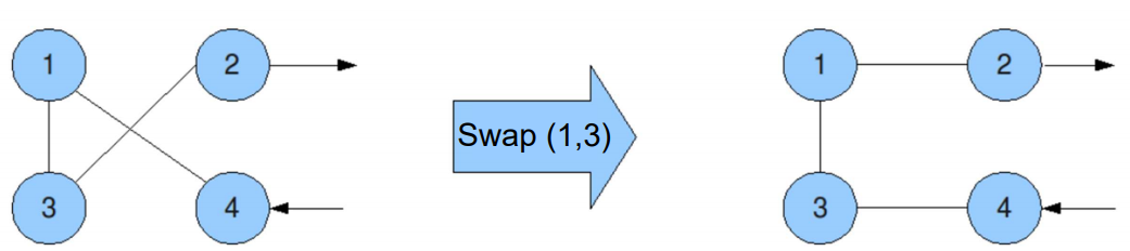
Permutation representation
- Useful in ordering/sequencing problems
- Task is (or can be solved by) arranging some objects in a certain order. Examples:
- production scheduling: important thing is which elements are scheduled before others (order)
- Travelling Salesman Problem (TSP) : important thing is which elements occur next to each other (adjacency)
- if there are n variables then the representation is as a list of n integers, each of which occurs exactly once
- Swap mutation
- Pick two alleles at random and swap their positions
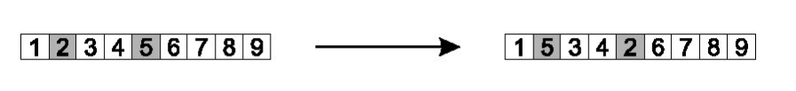
- Pick two alleles at random and swap their positions
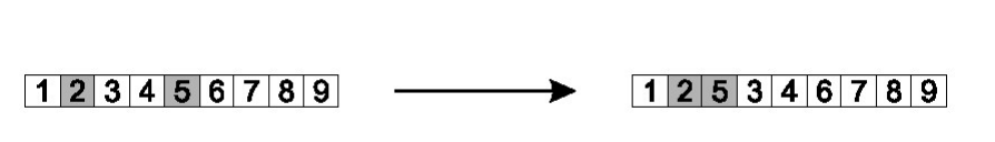
- Insert mutation
- Pick two allele values at random
- Move the second to follow the first, shifting the rest along to accommodate
- Note that this preserves most of the order and the adjacency information
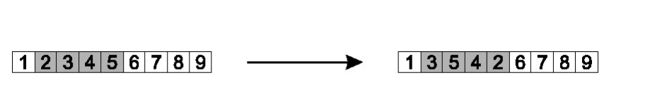
- Scramble mutation
- Pick a subset of genes at random
- Randomly rearrange the alleles in those positions
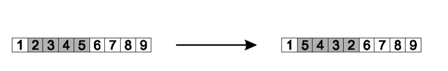
- Inversion mutation
- Pick two alleles at random and then invert the substring between them.
- Preserves most adjacency information (only breaks two links) but disruptive of order information
- Conserving Adjacency
- Important for problems where adjacency between elements decides quality (e.g. TSP)
- Partially Mapped Crossover and Edge Recombination are example operators

- Conserving Order
- Important for problems order of elements decide performance (e.g. production scheduling)
- Order Crossover and Cycle Crossover are example operators
Partially Mapped Crossover (PMX)
- Choose random segment and copy it from P1
- Starting from the first crossover point look for elements in that segment of P2 that have not been copied
- For each of these i look in the offspring to see what element j has been copied in its place from P1
- Place i into the position occupied j in P2, since we know that we will not be putting j there (as is already in offspring)
- If the place occupied by j in P2 has already been filled in the offspring k, put i in the position occupied by k in P2
- Having dealt with the elements from the crossover segment, the rest of the offspring can be filled from P2.
Second child is created analogously
def pmx(a,b,start,stop):
    child = [None]*len(a)

    child[start:stop] = a[start:stop]

    for ind, x in enumerate(b[start:stop]):
        ind += start
        if x not in child:
            while child[ind] != None:
                ind = b.index(a[ind])
            child[ind] = x

    for ind, x in enumerate(child):
        if x == None:
            child[ind] = b[ind]

    return child
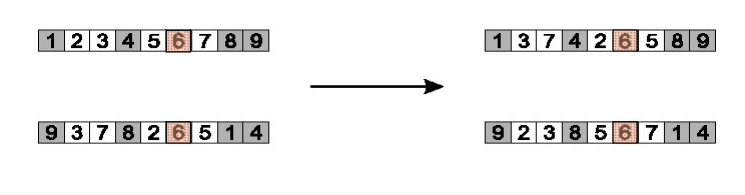
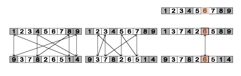
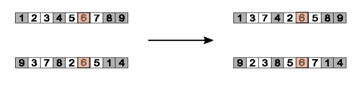
Edge Recombination
- Works by constructing a table listing which edges are present in the two parents, if an edge is common to both, mark with a +
- e.g. [1 2 3 4 5 6 7 8 9] and [9 3 7 8 2 6 5 1 4]
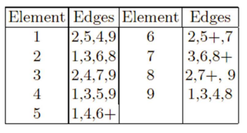
- e.g. [1 2 3 4 5 6 7 8 9] and [9 3 7 8 2 6 5 1 4]
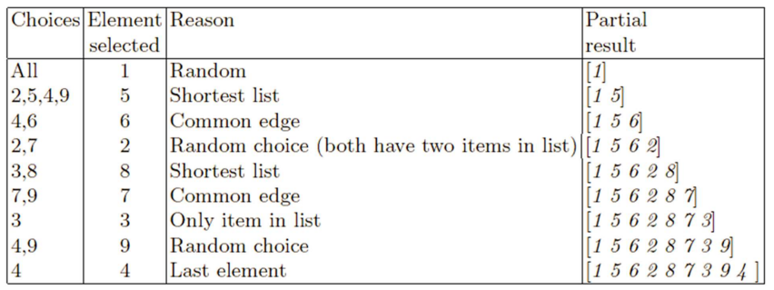
- Pick an initial element, entry, at random and put it in the offspring
- Set the variable current element = entry
- Remove all references to current element from the table
- Examine list for current element:
- If there is a common edge, pick that to be next element
- Otherwise pick the entry in the list which itself has the shortest list
- Ties are split at random
- In the case of reaching an empty list:
- a new element is chosen at random
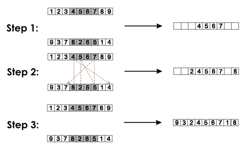
Order crossover
- Idea is to preserve relative order that elements occur
- Choose an arbitrary part from the first parent
- Copy this part to the first child
- Copy the numbers that are not in the first part, to the first child:
- starting right from cut point of the copied part,
- using the order of the second parent
- and wrapping around at the end
- Analogous for the second child, with parent roles reversed
- Copy randomly selected set from first parent
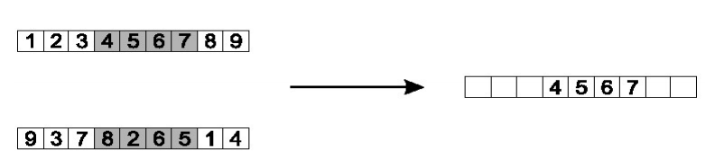
- Copy rest from second parent in order 1,9,3,8,2
def order_xover(a,b, start, stop):
    child = [None]*len(a)

    child[start:stop] = a[start:stop]

    b_ind = stop
    c_ind = stop
    l = len(a)
    while None in child:
        if b[b_ind % l] not in child:
            child[c_ind % l] = b[b_ind % l]
            c_ind += 1
        b_ind += 1
    return child
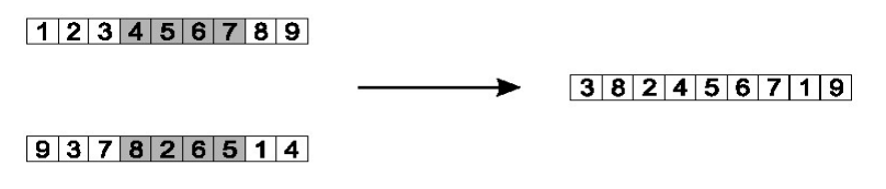
Cycle crossover
- Each allele comes from one parent together with its position.
- Make a cycle of alleles from P1 in the following way.
- Start with the first allele of P1.
- Look at the allele at the same position in P2
- Go to the position with the same allele in P1.
- Add this allele to the cycle.
- Repeat step b through d until you arrive at the first allele of P1.
- Put the alleles of the cycle in the first child on the positions they have in the first parent.
- Take next cycle from second parent
- Step 1: identify cycles
- Step 2: copy alternate cycles into offspring
def cycle_xover(a,b):
    child = [None]*len(a)
    while None in child:
        ind = child.index(None)
        indices = []
        values = []
        while ind not in indices:
            val = a[ind]
            indices.append(ind)
            values.append(val)
            ind = a.index(b[ind])
        for ind,val in zip(indices, values):
            child[ind] = val
        a,b = b,a
    return child
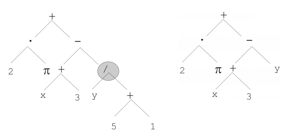
Tree Representation
- In Genetic Algorithms, Evolutionary Strategy and Evolutionary Programming chromosomes are linear structures (bit strings, integer string, real valued vectors, permutations)
- Tree shaped chromosomes are non-linear structures
- In GA, ES, EP the size of the chromosomes is fixed
- Trees in GP (Genetic Programming) may vary in depth and width
Mutation
- Most common mutation:
- replace randomly chosen subtree by randomly generated tree
- Mutation has two parameters:
- Probability \(p_m\) to choose mutation
- Probability to chose an internal point as the root of the subtree to be replaced
- Remarkably pm is advised to be 0 or very small, like 0.05
- The size of the child can exceed the size of the parent
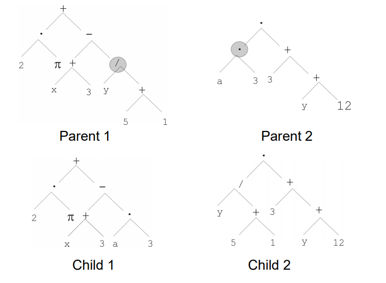
Recombination
- Most common recombination: exchange two randomly chosen subtrees among the parents
- Recombination has two parameters:
- Probability \(p_c\) to choose recombination
- Probability to chose an internal point within each parent as crossover point
- The size of offspring can exceed that of the parents
Fitness, Selection and Population Management
Population Management
- There are two main types:
- Generational model
- Each individual survive for one cycle
- \(\lambda\) offspring are generated
- The entire set of \(\mu\) parents are replaced by \(\mu\) offspring
- Steady-state model
- \(\lambda(<\mu)\) parents are replaced by \(\lambda\) offspring
- Generational model
- Generation Gap
- The proportion of the population replaced
- Parameter = 1.0 for Generational Model, = \(\lambda\)\pop_size for Steady-state model.
Fitness based competition
- Selection can occur in two places:
- Parent selection(selects mating pairs)
- Survivor selection(replaces population)
- Selection works on the population
- representation independent
- Selection pressure: As selection pressure increases, fitter solutions are more likely to survive, or be chosen as parents
- High selection pressure gives exploitation
- Low selection pressure gives exploration
Parent Selection
- Fitness-Proportionate Selection
- Higher fitness have a higher chance of being selected.
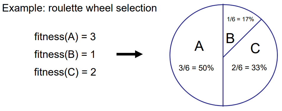
- Higher fitness have a higher chance of being selected.
- Stochastic Universal Sampling
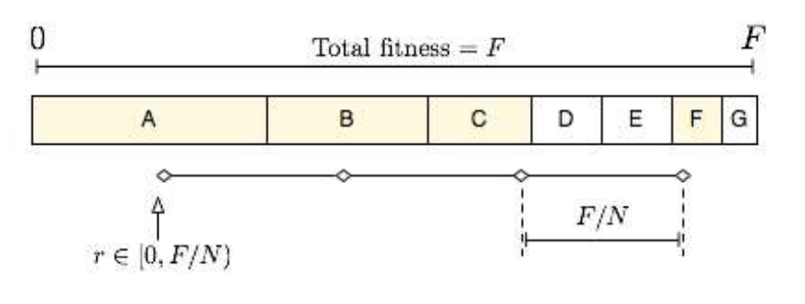
- “Select multiple individuals by making one spin of the wheel with a number of equally spaced arms”
Fitness-Proportionate Selection (FPS)
- Probability for individual i to be selected for mating in a population size μ with FPS is: \(P_{FPS}(i)=\frac{f_i}{\sum\limits_{j=1}^{\mu}f_j}\)
- Problems:
- Premature Convergence - one highly fit member can rapidly take over.
- Selection pressure lowers at the end of runs
- Scaling
- Windowing \(f’(i) = f(i)-\beta^t\) where \(\beta\) is the worst fitness in this(last n) generations
- Increases selection pressure
- Sigma Scaling \(f’(i) = max(f(i) - (\overline{f}-c\sigma_f),0)\) where *c is a constant, usually 2.0 (Normal distribution)
- Windowing \(f’(i) = f(i)-\beta^t\) where \(\beta\) is the worst fitness in this(last n) generations
Ranked-based selection
- Attempt to remove problems of FPS by basing selection probabilities on relative rather than absolute fitness
- Rank population according to fitness and then base selection probabilities on rank (fittest has rank μ-1 and worst rank 0)
- This imposes a sorting overhead on the algorithm
Tournament Selection
- All methods above rely on global population statistics
- Could be a bottleneck esp. on parallel machines, very large population
- Relies on presence of external fitness function which might not exist: e.g. evolving game players Idea for a procedure using only local fitness information:
- Pick k members at random then select the best of these
- Repeat to select more individuals
- Probability of selecting i will depend on:
- Rank of i
- Size of sample k
- higher k increases selection pressure
- Whether contestants are picked with replacement
- Picking without replacement increases selection pressure
- Whether fittest contestant always wins (deterministic) or this happens with probability p
Uniform
\(P_{uniform}(i)=\frac{1}{\mu}\)
- Parents are selected by uniform random distribution whenever an operator needs one/some
- Uniform parent selection is unbiased - every individual has the same probability to be selected
Survivor Selection(Replacement)
- From a set of μ old solutions and λ offspring:Select a set of μ individuals forming the next generation
- Survivor selection can be divided into two approaches:
- Age-Based Replacement
- Fitness is not taken into account
- Fitness-Based Replacement
- Usually with deterministic elements
- Age-Based Replacement
Fitness-based replacement
- Elitism
- Keep one copy, minimum, of the N fittest solution(s)
- Used in both GGA and SSGA
- Delete worst
- Replace \(\lambda\) worst individual* Delete worst
- Replace \(\lambda\) worst individuals
- Replace \(\lambda\) worst individual* Delete worst
- Round-robin tournament
- Pairwise competitions in round-robin format.
- x is evaluated against q other randomly chosen individuals(1v1)
- individuals are assigned “wins”
- solutions with most wins are winners
- Parameter q allows tuning selection pressure
- (\(mu,\lambda)\)-selection (best can be lost)
- only based on children \((\lambda > \mu)\)
- choose best offspring \(\mu\) for nest gen
- Most used because it is good at leaving local optima
- (\(mu+\lambda)\)-selection (elitist)
- based og parents and children
- based og parents and children
- chose the best offspring \(\mu\) for next gen
- based og parents and children
- Pairwise competitions in round-robin format.
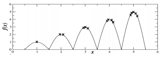
Multimodality
- The need for several local optima and solutions due to different strategies
Preserving Diversity
- Implicit approaches:
- Impose an equivalent of geographical separation
- Impose an equivalent of speciation
- Explicit approaches
- Make similar individuals compete for resource(fitness)
- Make similar individuals compete with each other for survival
Explicit approaches
- Fitness Sharing
- Restricts the number of individuals within a given niche by “sharing” their fitness
- Need to set the size of the niches share in either genotype or phenotype space
- run EA as normal but after each generation set
- Crowding
- Idea: New individuals replace similar individuals
- Randomly shuffle and pair parents, produce 2 offspring
- Each offspring competes with their nearest parent for survival (using a distance measure)
- Result: Even distribution among niches.
Implicit approaches
- Geographical Separation
- “Island” Model Parallel EA:
- Periodic migration of individual solutions between populations
- Run multiple populations in parallel
- After a (usually fixed) number of generations (an Epoch), exchange individuals with neighbours
- Repeat until ending criteria met
- Partially inspired by parallel/clustered systems
- Adaptively exchange individuals(stop pop when no improve over x gens)
- “Island” Model Parallel EA:
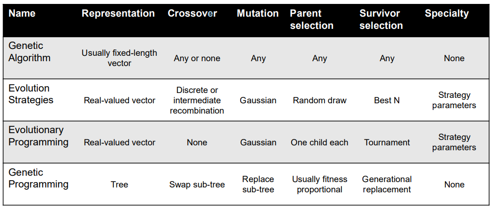
Popular Evolutionary Algorithm Variants
| Algorithm | Chromosome Representation | Crossover | Mutation |
|---|---|---|---|
| Genetic Algorithm (GA) | Array | X | X |
| Genetic Programming (GP) | Tree | X | X |
| Evolution Strategies (ES) | Array | (X) | X |
| Evolutionary Programming (EP) | No Constraints | - | X |
Genetic Algorithms
Simple GA
- Typically applied to:
- discrete function optimization
- benchmark for comparison with other algorithms
- straightforward problems with binary representation
- Features:
- not too fast
- missing new variants (elitism, sus)
- often modelled by theorists
- Reproduction cycle:
- Select parents for the mating pool (size of mating pool = population size)
- Shuffle the mating pool
- Apply crossover for each consecutive pair with probability pc, otherwise copy parents
- Apply mutation for each offspring (bit-flip with probability pm independently for each bit)
- Replace the whole population with the resulting offspring
| Summary | |
|---|---|
| Representation | Bit-strings |
| Recombination | 1-Point Crossover |
| Mutation | Bit flip |
| Parent selection | Fitness proportional – implemented by Roulette Wheel |
| Survivor selection | Generational |
Genetic Programming GP
- Typically applied to:
- machine learning tasks (prediction, classification…)
- Attributed features:
- “automatic evolution of computer programs”
- needs huge populations (thousands)
- slow
- Special
- non-linear chromosomes: trees
- mutation possible but not necessary
- Tree Representation
- Non-linear
- Variable size
- Mutation
- The trees have a tendency to bloat as the average population increases over time
- Countermeasures:
- Maximum tree size
- Parsimony pressure: penalty for being oversized
- Countermeasures:
| Summary | |
|---|---|
| Representation | Tree structures |
| Recombination | Exchange of subtrees |
| Mutation | Random change in trees |
| Parent selection | Fitness proportional |
| Survivor selection | Generational replacement |
Evolution Strategies ES
- Attributed features:
- fast
- good optimizer for real-valued optimisation
- relatively much theory
- Special:
- self-adaptation of (mutation) parameters standard
- Representation:
- Chromosomes consist of two parts:
- Object variables: \(x_1,…,x_n\)
- Strategy parameters (mutation rate, etc): \(p_1,…,p_n\)
- Full size: \({x_1,…,x_n,p_1,…p_n}\)
- Chromosomes consist of two parts:
- Parent selection
- Parents are selected by uniform random distribution whenever an operator needs one/some
- Thus: ES parent selection is unbiased - every individual has the same probability to be selected \(P_{uniform}(i)=\frac{1}{\mu}\)
- Recombination
- Two parents create one child
- Acts per variable / position by either
- Intermediary crossover(1,1,1)+(2,2,2)=(1,2,1)
- Discrete crossover(1,1,1)+(2,2,2)=(1.5,1.5,1.5)
- From two or more parents by either:
- Local recombination: Two parents make a child
- Global recombination: Selecting two parents randomly for each gene
| Two fixed parents | Two parents selected for each i |
|---|---|
| Local intermediary | Global intermediary |
| Local discrete | Global discrete |
| Summary | |
|---|---|
| Representation | Real-valued vectors |
| Recombination | Discrete or intermediary |
| Mutation | Gaussian perturbation |
| Parent selection | Uniform random |
| Survivor selection | \((\mu,\lambda) \text{or} (\mu+\lambda)\) |
Evolutionary Programming EP
- Typically applied to:
- traditional EP: prediction by finite state machines
- contemporary EP: (numerical) optimization
- Attributed features:
- very open framework: any representation and mutation op’s OK
- Contemporary EP has almost merged with ES
- Special:
- no recombination
- self-adaptation of parameters standard (contemporary EP)
- Representation
- For continuous parameter optimisation
- Chromosomes consist of two parts:
- Object variables: \(x_1,…,x_n\)
- Mutation step sizes: \(\sigma_1,…,\sigma_n\)
- Full size: \(\langle x_1,…,x_n, \sigma_1,…,\sigma_n\rangle\)
- Selection
- Each individual creates one child by mutation
- Deterministic
- Not biased by fitness
- Parents and offspring compete for survival in round-robin tournaments.
- Each individual creates one child by mutation
| Summary | |
|---|---|
| Representation | Real-valued vectors |
| Recombination | None |
| Mutation | Gaussian perturbation |
| Parent selection | Deterministic (each parent one offspring) |
| Survivor selection | Probabilistic \((\mu+\lambda)\) |
Summary
Working with Evolutionary Algorithms
Typical applications for EAs
- Design Problem
- Optimising spending on improvements to national road network
- Computing costs negligible
- Six months to run algorithm on hundreds computers
- Many runs possible
- Must produce very good result just once
- Optimising spending on improvements to national road network
- Repetitive Problem
- Optimising Internet shopping delivery route
- Need to run regularly/repetitively
- Different destinations each day
- Limited time to run algorithm each day
- Must always be reasonably good route in limited time
- Optimising Internet shopping delivery route
- On-Line Control
- Darpa Robot Competition
- Need to run regularly/repetitively
- Limited time to run algorithm
- Must always deliver reasonably good solution in limited time
- Darpa Robot Competition
Academic Research on EAs
- Show that EC is applicable in a (new) problem domain (real-world applications)
- Show that my_EA is better than benchmark_EA
- Show that EAs outperform traditional algorithms
- Optimize or study impact of parameters on the performance of an EA
- Investigate algorithm behavior (e.g. interaction between selection and variation)
- See how an EA scales-up with problem size
- ..
Algorithm design
- Design a representation
- Design a way of mapping a genotype to a phenotype
- Design a way of evaluating an individual
- Design suitable mutation operator(s)
- Design suitable recombination operator(s)
- Decide how to select individuals to be parents
- Decide how to select individuals for the next generation (how to manage the population)
- Decide how to start: initialization method
- Decide how to stop: termination criterion
Measurements and statistics
Basic rules of experimentation
- EAs are stochastic -> never draw any conclusion from a single run
- perform sufficient number of independent runs
- use statistical measures (averages, standard deviations)
- use statistical tests to assess reliability of conclusions
- EA experimentation is about comparison -> always do a fair competition
- use the same amount of resources for the competitors
- try different comp. limits (to cope with turtle/hare effect)
- use the same performance measures
How to Compare EA Results?
- Success Rate: Proportion of runs within x% of target
- Mean Best Fitness: Average best solution over n runs
- Best result (“Peak performance”) over n runs
- Worst result over n runs
Peak vs Average Performance
- For repetitive tasks, average (or worst) performance is most relevant
- For design tasks, peak performance is most relevant
Measures
- Performance measures(off-line)
- Efficiency (alg. speed)
- Execution time
- Average no. of evaluations to solution (AES, i.e., number of generated points in the search space)
- Effectiveness (solution quality, also called accuracy)
- Success rate (SR): % of runs finding a solution
- Mean best fitness at termination (MBF)
- “Working” measures (on-line)
- Population distribution (genotypic)
- Fitness distribution (phenotypic)
- Improvements per time unit or per genetic operator
- Efficiency (alg. speed)
Statistical Comparisons and Significance
- If a claim is made “Mutation A is better than mutation B”, need to show statistical significance of comparisons
- Fundamental problem: two series of samples (random drawings) from the SAME distribution may have DIFFERENT averages and standard deviations
- Tests can show if the differences are significant or not
- Standard deviations supply additional info
- T-test (and alike) indicate the chance that the values came from the same underlying distribution (difference is due to random effects).
Summary for experiments
- Be organized
- Decide what you want & define appropriate measures
- Choose test problems carefully
- Make an experiment plan (estimate time when possible)
- Perform sufficient number of runs
- Keep all experimental data (never throw away anything)
- Include in publications all necessary parameters to make others able to repeat your experiments
- Use good statistics (“standard” tools from Web, MS, R)
- Present results well (figures, graphs, tables, …)
- Watch the scope of your claims
- Aim at generalizable results
- Publish code for reproducibility of results (if applicable)
- Publish data for external validation (open science)
Hybridisation with Other Techniques
Memetic Algorithms
- What is it?
- The combination of Evolutionary Algorithms with Local Search Operators that work within the EA loop has been termed “Memetic Algorithms”
- Term also applies to EAs that use instance specific knowledge
- Memetic Algorithms have been shown to be orders of magnitude faster and more accurate than EAs on some problems, and are the “state of the art” on many problems.
Reasons to hybridise
- Might be looking at improving on existing techniques (non-EA)
- Might be looking at improving EA search for good solutions
Local Search
Main Idea simplified
- Make a small, but intelligent (problem-specific), change to an existing solution
- If the change improves it, keep the improved version
- Otherwise, keep trying small, smart changes until it improves, or until we have tried all possible small changes
Def
- Defined by combination of neighbourhood and pivot rule
- N(x) is defined as the set of points that can be reached from x with one application of a move operator
- e.g. bit flipping search on binary problems
Pivot rules
- Is the neighbourhood searched randomly, systematically or exhaustively
- does the search stop as soon as a fitter neighbour is found (Greedy Ascent)
- or is the whole set of neighbours examined and the best chosen (Steepest Ascent)
- of course there is no one best answer, but some are quicker than others to run …
Evolution
- Do offspring inherit what their parents have “learnt” in life?
- Yes - Lamarckian evolution
- Traits acquired in parents lifetimes can be inherited by offspring
- Improved fitness and genotype
- No - Baldwinian evolution
- Improved fitness only
- Yes - Lamarckian evolution
- In practice, most recent Memetic Algorithms use:
- Pure Lamarckian evolution, or
- A stochastic mix of Lamarckian and Baldwinian evolution
Where to hybridise
Summary
- It is common practice to hybridise EA’s when using them in a real world context
- This may involve the use of operators from other algorithms which have already been used on the problem, or the incorporation of domain-specific knowledge
- Memetic algorithms have been shown to be orders of magnitude faster and more accurate than EAs on some problems, and are the “state of the art” on many problems
Multiobjective Evolutionary Algorithms
MOPs - Multi-Objective Problems
- Wide range of problems can be categorise by the presence of a number of n possibly conflicting objectives:
- buying a car: speed vs. price vs. reliability
- engineering design: lightness vs. strength
- Two problems:
- finding set of good solutions
- choice of best for the particular application
Two approaches to multiobjective optimisation
- Weighted sum (scalarisation):
- transform into a single objective optimisation method
- compute a weighted sum of the different objectives
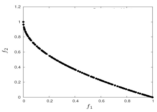
- A set of multi-objective solutions (Pareto front):
- The population-based nature of EAs used to simultaneously search for a set of points approximating Pareto front
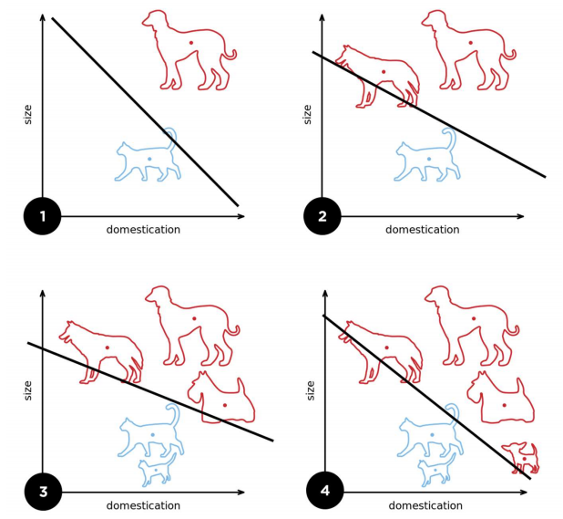
Comparing solutions
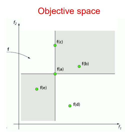
- Minimization:
- a is better than b
- a is better than c
- a is worse than e
- a and d are incomparable
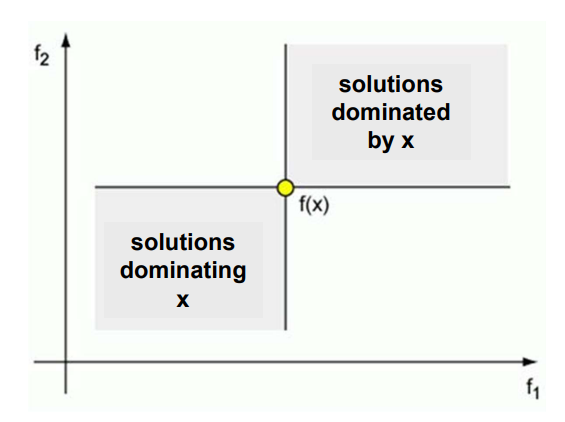
Dominance relation
- Solution x dominates solution y, \(x \preceq y\) if:
- x is better than y in at least one objective,
- x is not worse than y in all other objectives
Pareto optimality
- Solution x is non-dominated among a set of solutions Q if no solution from Q dominates x
- A set of non-dominated solutions from the entire feasible solution space is the Pareto set, or Pareto front, its members Pareto-optimal solutions
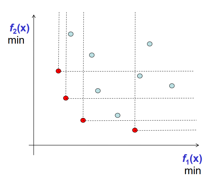
Goal of multiobjective optimisers
- Find a set of non-dominated solutions (approximation set) following the criteria of:
- convergence (as close as possible to the Pareto optimal front),
- diversity (spread, distribution)
EC approach:
- Requirements:
- Way of assigning fitness and selecting individuals, usually based on dominance
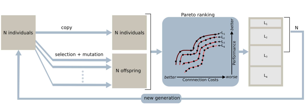
- Preservation of a diverse set of points, similarities to multi-modal problems
- Aim: Evenly distributed population along the Pareto front
- Usually done by niching techniques such as:
- fitness sharing
- adding amount to fitness based on inverse distance to nearest neighbour
- All rely on some distance metric in genotype /phenotype / objective space
- Remembering all the non-dominated points you have seen, usually using elitism or an archive
- Could just use elitist algorithm, e.g. \( \mu + \lambda \) replacement
- Common to maintain an archive of non dominated points
- some algorithms use this as a second population that can be in recombination etc.
- Way of assigning fitness and selecting individuals, usually based on dominance
Summary
- MO problems occur very frequently
- EAs are very good in solving MO problems
- MOEAs are one of the most successful EC subareas
Machine learning and single-layer neural networks
What ML is
- A program that can learn from experience
- Modify execution based on new information
- Analyzing new data by applying known relevant information
When should ML be used
- Human expertise does not exist (navigating on Mars)
- Humans are unable to explain their expertise (speech recognition)
- Solution changes over time (self-driving vehicles)
- Solution needs to be adapted to particular cases (user preferences)
- Interfacing computers with the real world (noisy data)
- Dealing with large amounts of (complex) data
Types of ML
Supervised learning: Training data include desired outputs. Based on this training set, the algorithm generalises to respond correctly to all possible inputs.
- Unsupervised learning: Training data does not include desired outputs, instead the algorithm tries to identify similarities between the inputs that have something in common so that similar items are categorised together.
- Reinforcement learning: The algorithm is told when the answer is wrong, but does not get told how to correct it. Algorithm must balance exploration of the unknown environment with exploitation of immediate rewards to maximize long-term rewards.
Supervised learning
- Training data provided in pai
- Goal is to predict output(y) to input (x): \(y = f(x)\)
- Supervision part is output y for each input x.
- Examples:
- Classification
- Regression
Classification
- Training data consists of “inputs”, denoted x, and corresponding output “class labels”, denoted as y
- Goal is to correctly predict for a test data input the corresponding class label.
- Learn a “classifier” f(x) from the input data that outputs the class label or a probability over the class labels.
- Example:
- Input: image
- Output: category label, eg “cat” vs. “no cat”
- Two main phases:
- Training: Learn the classification model from labeled data.
- Prediction: Use the pre-built model to classify new instances.
- Classification creates boundaries in the input space between areas assigned to each class
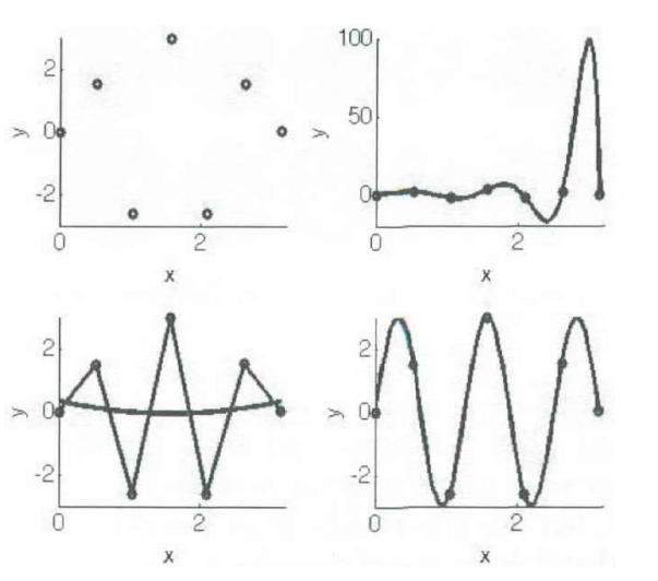
Regression
- Regression analysis is used to predict the value of on variable (the dependent variable) on the basis of other variables (the independent variables).
- Learn a continuous function.
- Given, the following data, can we find the value of the output when x = 0.44?
- Goal is to predict for input x an output f(x) that is close to the true y.
- It is generally a problem of function approximation, or interpolation, working out the value between values that we know.
Machine Learning Process
- Data Collection and Preparation
- Feature Selection and Extraction
- Algorithm Choice
- Parameters and Model Selection
- Training
- Evaluation
McCulloch and Pitts Neurons
- Sum the weighted inputs
- If total is greater than some threshold, neuron “fires”
- Otherwise does not
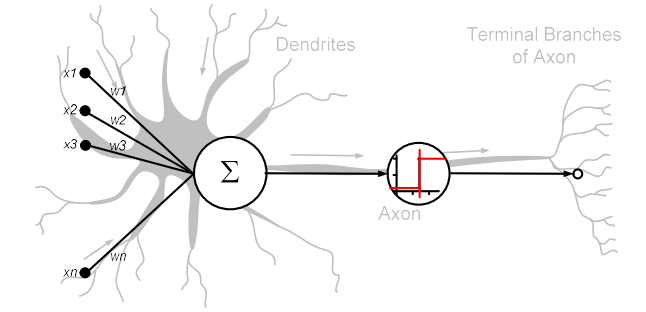
\(h = \sum_{i=1}^{m} x_i w_i \qquad o = \left. \begin{cases} 1 & h \geq \theta \\ 0 & h < \theta \end{cases} \right\}\)
- The weight \(w_j\) can be positive or negative
- Inhibitory or exitatory.
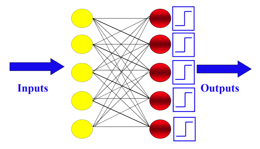
Neural Networks
- Can put lots of McCulloch & Pitts neurons together.
- Connect them up in any way we like.
- In fact, assemblies of the neurons are capable of universal computation.
- Can perform any computation that a normal computer can.
- Just have to solve for all the weights \(w_{ij}\)
The Perceptron Network
- Training neurons is done by adapting the weights
- Supervised learning with target outputs.
Learning rule:
\(w_{ij} \leftarrow w_{ij} + \Delta w_{ij}\)
- Aim: minimize the error at the output
- If E = t-y, want E to be 0
- Use: \(\Delta w = \eta(t_j + y_j)x_i\)
- Learning rate: \(\eta\)
- controls the size of the weight changes
- Big LR might overshoot, small LR learns slower.
- Desired output: \(t_j\)
- Actual output: \(y_j\)
- Error: \(t_j + y_j\)
- Input: \(x_i\)
- Learning rate: \(\eta\)
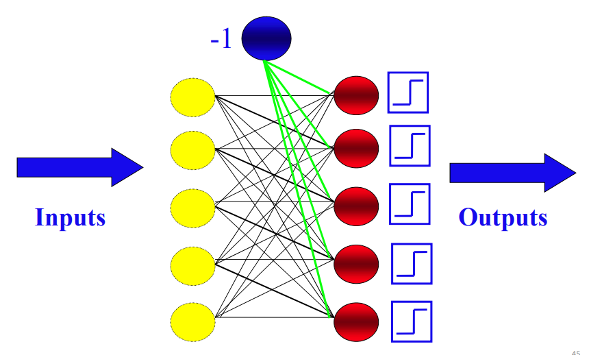
Bias input
- A fix to make the neuron learn what output to give, when all inputs are zero.
- Add each neuron an extra input with a fixed value: A bias node
Limitations
- A single layer perceptron can only learn linearly separable problems.
- Boolean AND function is linearly separable, whereas Boolean XOR function is not.
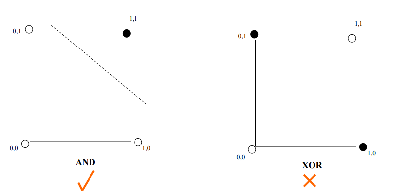
- Boolean AND function is linearly separable, whereas Boolean XOR function is not.
Multi-Layer Network
- A neural network with one or more layers of nodes between the input and the output nodes is called multilayer network
- The multilayer network structure, or architecture, or topology, consists of an input layer, one or more hidden layers, and one output layer.
- The input nodes pass values to the first hidden layer, its nodes to the second and so until producing outputs.
- A network with a layer of input units, a layer of hidden units and a layer of output units is a two-layer network.
- A network with two layers of hidden units is a three layer network, and so on.
Multi-Layer Perceptron(MPL)
- No connections within a single layer.
- No direct connections between input and output layers
- Number of output units need not equal number of input units.
- Number of hidden units per layer can be more or less than input or output units.
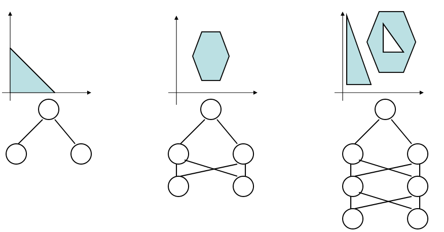
Layers
- draws linear boundaries
- combines the boundaries
- generate arbitrarily complex boundaries
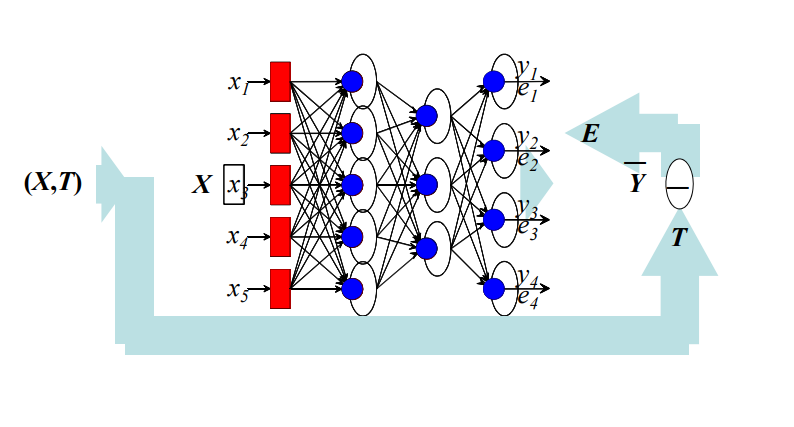
Backpropagation Algorithm
- Forward step: Propagate activation from input to output layer
- Put the input values in the input layer
- Calculate the activations of the hidden nodes
- Calculate the activations of the output nodes
- Backward step: propagate errors from output to hidden layer
- Calculate the output errors
- Update last layer of weights
- Propagate error backward, update hidden weights
- Until first layer is reached
Error Function
- Single scalar function for entire network
- Parameterized by weights (objects of interest)
- Multiple errors of different signs should not cancel out
- Sum-of-squares error:
- \[E(w) = \frac{1}{2}\sum_k(t_k-y_k)^2=\frac{1}{2}\sum_k(t_k-\sum_iw_{ik}x_i)^2\]
Gradient Descent Learning
- Compute gradient \(\rightarrow\) differentiate sum-of squares error function
- \[\Delta w_{ik} = -\eta\frac{\partial E}{\partial w_{ik}}\]
Error terms
- For the outputs
- \[\delta_k = (y_k-t_k)g'(a_k)\]
- For the hidden nodes
- \[\delta_j = g'(u_j)\sum_k \delta_k w_{jk}\]
Update Rules
- For the weights connected to the outputs:
- \[w_{jk} \leftarrow w_{jk}-\eta\delta_kz_j\]
- For the weights on the hidden nodes:
- \[v_{ij} \leftarrow v_{ij}-\eta\delta_jz_i\]
- The learning rate \(\eta\) depends on the application
Algorithm (sequential)
- Apply an input vector and calculate all activations, a and u
- Evaluate deltas for all output units:
- \[\delta_k = (y_k-t_k)g'(a_k)\]
- Propagate deltas backwards to hidden layer deltas:
- \[\delta_j = g'(u_j)\sum_k \delta_k w_{jk}\]
- Update weights:
- \[w_{jk} \leftarrow w_{jk}-\eta\delta_kz_j\]
- \(v_{ij} \leftarrow v_{ij}-\eta\delta_jz_i\)
Activation function
- Defines the output of a node given a input or set og inputs.
- Must be nonlinear, differentiable and have a bounded range
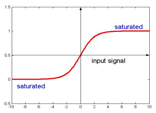
Sigmoidal Function
- Common in MLP
- \[g(a_i) = \frac{1}{1+exp(-ka_i)} = \frac{1}{1+e^{-ka_i}}\]
- k is a positive constant.
- Range from 0 to 1.
- Can use tanh(ka), same shape but range from -1 to 1.
Network Training
Batch Training
- Update weights after all inputs seen
- Need many epochs
- One loop through all the training data is called an epoch
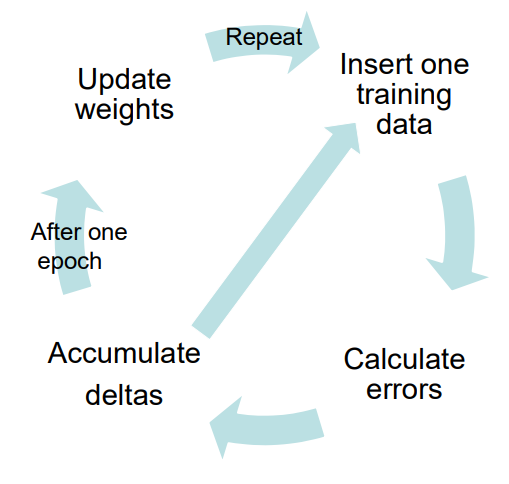
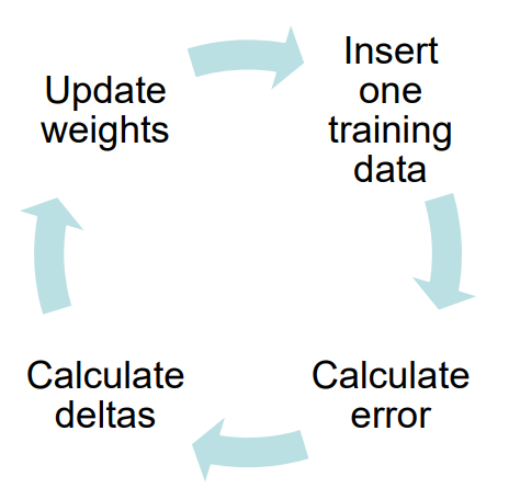
Sequential Training
- Update weights after each input is seen
- Need many epochs
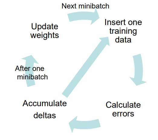
Minibatch
- Split all data into N minibatches
- Feed each minibatch to the network
- Shuffle data and repeat
- May lead to the benefits of both batch-learning and sequential learning:
- Rapid convergence
- Avoiding local minima
Avoiding local minimum/optimum
- Initialize training many times with random weights
- Use momentum:
- \[w_{ij} \leftarrow w_{ij} - \eta\Delta_jz_i+\alpha\Delta w_{ij}^{t-1}\]
Practical Issues
Amount of Training
- Use 10 times more data than the number of weights
Generalization
- Aim of nerual network learning: Generalise from training examples to all possible inputs.
-
The objective of learning is to achieve good generalization to new cases; we cannot train on all possible data.
- Underfitting:
- Symptoms:
- High training error
- Training error close to test error
- High bias
- Possible remedies:
- Complexify model
- Add more features
- Train longer
- Symptoms:
- Just right:
- Symptoms:
- Training error slightly lower than test error
- Symptoms:
- Overfitting:
- Symptoms:
- Very low training error
- Training error much lower than test error
- High variance
- Possible remedies:
- Perform regularization
- Get more data
- Symptoms:
- Approximation of \(y = f(x)\):

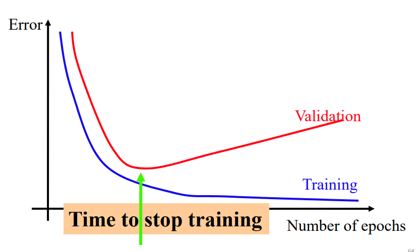
Overfitting solution - Cross-Validation
To maximize generalization and avoid overfitting, split data into three sets:
- Training set: Train the model.
- Validation set: Judge the model’s generalization ability during training.
- Test set: Judge the model’s generalization ability after training.
Validation set
- Data unseen by training algorithm – not used for backpropagation.
- Network is not trained on this data, so we can use it to measure generalization ability.
- Goal is to maximize generalization ability, so we should minimize the error on this data set.
Testing set
- Data unseen during training and validation.
- Has no influence on when to stop training.Has no influence on when to stop training.
- With early stopping, we’ve maximized the ability to generalize to the validation set;
- To judge the final result, we should measure its ability to generalize to completely unseen data.
Reinforcement Learning
An agent has a state, and based on its actions it relives rewards/punishment. The goal is to learn actions that maximize reward.
- Learning is guided by the reward
- An infrequent numerical feedback indicating how well we are doing.
- Problems:
- The reward does not tell us what we should have done!
- The reward may be delayed – does not always indicate when we made a mistake.
The reward Function
- Corresponds to the fitness function of an evolutionary algorithm.
- \(r_{t+1}\) is a function of \((s_t, a_t)\)
- The reward is a numeric value, and can be negative(punishment).
- Can be given throughout the learning episode, or only in the end.
- Goal is to maximize total reward.
Maximizing total reward
- Total reward: \(\sum\limits_{t=0}^{N-1} r_{t+1}\)
Future rewards may be uncertain and we might care more about rewards that come soon. Therefore, we discount future rewards:
-
\(R = \sum\limits_{t=0}^{\infty} \gamma^t t_{t+1}, \qquad 0 \leq \gamma \leq 1\) or \(R = \sum\limits_{k=0}^{\infty} \gamma^k r_{t+k+1}, \qquad 0 \leq \gamma \leq 1\)
- Future reward: \(R = r_1 + r_2 + ... + r_n\) \(R_t = r_t + r_{t+1} + ... + r_n\)
- Discount future rewards
- A good strategy for an agent would be to always choose an action that maximizes the (discounted) future reward.
Action Selection
- At each learning stage, the RL algorithm looks at the possible actions and calculates the expected average reward.
- Based on \(Q_{s,t}(a)\), an action will be selected using:
- Greedy strategy: pure exploitation
- \(epsilon\)-Greedy strategy: exploitation with a little exploration
- Soft-Max strategy: \(P(Q_{s,t}(a)) = \frac{e^{Q_{s,t}(a)/\tau}}{\sum_b e^{Q_{s,t}(b)/\tau}}\)
Policy \((\pi)\) and Value (\(V\))
- The set of actions we took define our policy.\((\pi)\)
- The expected rewards we get in return, defines our value (\(V\)).
Markov Decision Process
- If we only need to know the current state, the problem has the Markov property**.
- No Markov Property:
- \[P_r ( r_t = r',s_{s+t} = s'|s_t,a_t,r_{t-1},...,r_1,s_1,a_1,S_0,a_0 )\]
- Markov property:
- \[P_r(r_t = r',s_{t+1} = s'|s_t,a_t)\]
Value
- The expected future reward is known as the value.
- Two ways to compute the value:
- The value of a state, \(V(s)\), averaged over all possible actions in that state.
- (state-value function)
- \[V(s) = E(r_t|s_t = s) = E(\sum_{i_0}^{\infty} \gamma^t r_{t+i+1} | s_t = s)\]
- (state-value function)
- The value of a state/action pair \(Q(s,a)\).
- (action-value function)
- \[Q(s,a) = E(r_t | s_t = s,a_t = a) = E(\sum_{i_0}^{\infty} \gamma^t r_{t+i+1} | s_t = s, a_t = a)\]
- (action-value function)
- The value of a state, \(V(s)\), averaged over all possible actions in that state.
- Q and V are initially unknown, and learned iteratively as we gain experience
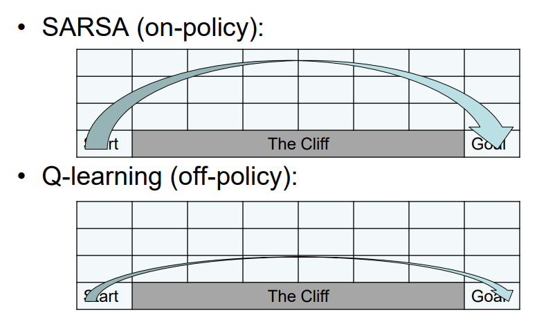
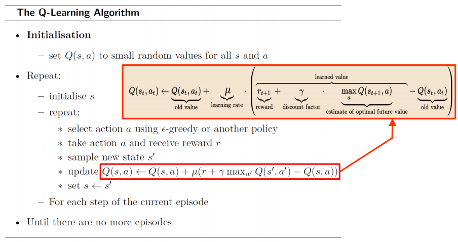
The Q-Learning Algorithm
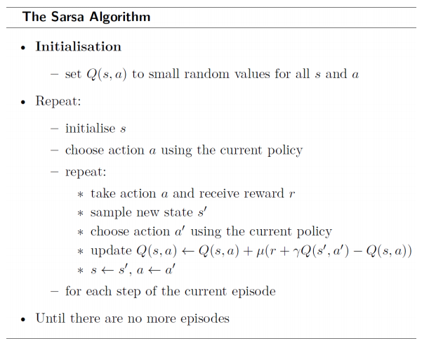
The SARSA Algorithm
On-policy vs off-policy learning: